Bulk Theory
Bulk phase diagrams enable the comparison of the thermodynamic stability of various different bulk phases under different chemical potentials giving valuable insight in to the syntheis of solid phases.
This theory example will consider a series of bulk phases which can be defined through a reaction scheme across all phases,
thus for this example including MgO,  and
and  as reactions and A as a generic product.

The system is in equilibrium when the chemical potentials of the reactants and product are equal; i.e. the change in Gibbs free energy is  .
.

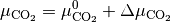
Assuming that and are gaseous species,  and
and  can be written as
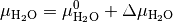
and
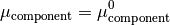
The chemical potential  is the partial molar free energy of any reactants or products (x) in their standard states,
in this example we assume all solid components can be expressed as
is the partial molar free energy of any reactants or products (x) in their standard states,
in this example we assume all solid components can be expressed as
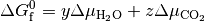
Hence, we can now rearrange the equations to produce;

As  corresponds to the partial molar free energy of product A, we can replace the left side with the Gibbs free energy (
 ).
).

At equilibrium , and hence
Thus, we can find the values of  and
and  (or
(or  and
and  when Mg-rich phases are in thermodynamic equilibrium; i.e.
they are more or less stable than MgO.
This procedure can then be applied to all phases to identify which is the most stable, provided that the free energy
when Mg-rich phases are in thermodynamic equilibrium; i.e.
they are more or less stable than MgO.
This procedure can then be applied to all phases to identify which is the most stable, provided that the free energy  is known for each Mg-rich phase.
The free energy can be calculated using

Where for this example the free energy (G) is equal to the calculated DFT energy ( ).
).
Temperature
The previous method will generate a phase diagram at 0 K. This is not representative of normal conditions. Temperature is an important consideration for materials chemistry and we may wish to evaluate the phase thermodynamic stability at various synthesis conditions.
As before the free energy can be calculated using;
Where for this exmaple the free energy (G) for solid phases is equal to is equal to the calculated DFT energy  .
For gaseous species, the standard free energy varies significantly with temperature, and as DFT simulations are designed for condensed phase systems,
we use experimental data to determine the temperature dependent free energy term for gaseous species, where
.
For gaseous species, the standard free energy varies significantly with temperature, and as DFT simulations are designed for condensed phase systems,
we use experimental data to determine the temperature dependent free energy term for gaseous species, where  is specific entropy value for a given T and
  is the,
both can be obtained from the NIST database and can be calculated as;
is the,
both can be obtained from the NIST database and can be calculated as;

Pressure
In the previous tutorials we went through the process of generating a simple phase diagram for bulk phases and introducing temperature dependence for gaseous species. This useful however, sometimes it can be more beneficial to convert the chemical potenials (eVs) to partial presure (bar).
Chemical potential can be converted to pressure values using

where P is the pressure,  is the chemical potential of oxygen, $k_B$ is the Boltzmnann constant and T is the temperature.