Chemical Potential¶

The physical quantity that is used to define the stability of a surface with a given composition is its surface energy $\gamma$ (J $m^{-2}$ ). At its core, surfinpy is a code that calculates the surface energy of different slabs and uses these surface energies to build a phase diagram. In this explantion of theory we will use the example of water adsorbing onto a surface of $TiO_2$ containing oxygen vacancies. In such an example there are two variables, water concentration and oxygen vacancy concentration. We are able to calculate the surface energy according to

$\gamma_{Surf} = \frac{1}{2A} \Bigg( E_{TiO_2}^{slab} - \frac{nTi_{slab}}{nTi_{Bulk}} E_{TiO_2}^{Bulk} \Bigg) - \Gamma_O \mu_O - \Gamma_{H_2O} \mu_{H_2O} ,$

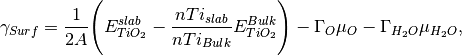
where A is the surface area, $E_{TiO_2}^{slab}$ is the DFT energy of the slab, $nTi_{Slab}$ is the number of cations in the slab, $nTi_{Bulk}$ is the number of cations in the bulk unit cell, $E_{TiO_2}^{Bulk}$ is the DFT energy of the bulk unit cell and

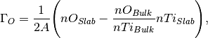
$\Gamma_O = \frac{1}{2A} \Bigg( nO_{Slab} - \frac{nO_{Bulk}}{nTi_{Bulk}}nTi_{Slab} \Bigg) ,$

$\Gamma_{H_2O} = \frac{nH_2O}{2A} ,$

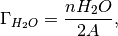
where $nO_{Slab}$ is the number of anions in the slab, $nO_{Bulk}$ is the number of anions in the bulk and $nH_2O$ is the number of adsorbing water molecules. $\Gamma_O$ / $\Gamma_{H_2O}$ is the excess oxygen / water at the surface and $\mu_O$ / $\mu_{H_2O}$ is the oxygen / water chemcial potential. Clearly $\Gamma$ and $mu$ will only matter when the surface is non stoichiometric.

Usage¶

The first thing to do is input the data that we have generated from our DFT calculations. The input data needs to be contained within a dictionary. First we have created the dictionary for the bulk data, where Cation is the number of cations, Anion is the number of anions, Energy is the DFT energy and F-Units is the number of formula units.

bulk = {'Cation' : Cations in Bulk Unit Cell,
        'Anion' : Anions in Bulk Unit Cell,
        'Energy' :  Energy of Bulk Calculation,
        'F-Units' : Formula units in Bulk Calculation}

Next we create the slab dictionaries - one for each slab calculation or “phase”. Cation is the number of cations, X is in this case the number of oxygen species (corresponding to the X axis of the phase diagram), Y is the number of in this case water molecules (corresponding to the Y axis of our phase diagram), Area is the surface area, Energy is the DFT energy, Label is the label for the surface (appears on the phase diagram) and finally nSpecies is the number of adsorbing species (In this case we have a surface with oxygen vacancies and adsorbing water molecules - so nSpecies is 1 as oxygen vacancies are not an adsorbing species, they are a constituent part of the surface).

surface = {'Cation': Cations in Slab,
           'X': Number of Species X in Slab,
           'Y': Number of Species Y in Slab,
           'Area': Surface area in the slab,
           'Energy': Energy of Slab,
           'Label': Label for phase,
           'nSpecies': How many species are non stoichiometric}

This data needs to be contained within a list. Don’t worry about the order, surfinpy will sort that out for you.

We also need to declare the range in chemical potential that we want to consider. Again these exist in a dictionary. Range corresponds to the range of chemcial potential values to be considered and Label is the axis label.

deltaX = {'Range': Range of Chemical Potential,
          'Label': Species Label}

from surfinpy import mu_vs_mu

bulk = {'Cation' : 1, 'Anion' : 2, 'Energy' : -780.0, 'F-Units' : 4}

pure =     {'Cation': 24, 'X': 48, 'Y': 0, 'Area': 60.0,
            'Energy': -575.0,   'Label': 'Stoich',  'nSpecies': 1}
H2O =      {'Cation': 24, 'X': 48, 'Y': 2, 'Area': 60.0,
            'Energy': -612.0,   'Label': '1 Water', 'nSpecies': 1}
H2O_2 =    {'Cation': 24, 'X': 48, 'Y': 4, 'Area': 60.0,
            'Energy': -640.0,   'Label': '2 Water', 'nSpecies': 1}
H2O_3 =    {'Cation': 24, 'X': 48, 'Y': 8, 'Area': 60.0,
            'Energy': -676.0,   'Label': '3 Water', 'nSpecies': 1}
Vo =       {'Cation': 24, 'X': 46, 'Y': 0, 'Area': 60.0,
            'Energy': -558.0,   'Label': 'Vo', 'nSpecies': 1}
H2O_Vo =   {'Cation': 24, 'X': 46, 'Y': 2, 'Area': 60.0,
            'Energy': -594.0,  'Label': 'Vo + 1 Water', 'nSpecies': 1}
H2O_Vo_2 = {'Cation': 24, 'X': 46, 'Y': 4, 'Area': 60.0,
            'Energy': -624.0,  'Label': 'Vo + 2 Water', 'nSpecies': 1}
H2O_Vo_3 = {'Cation': 24, 'X': 46, 'Y': 6, 'Area': 60.0,
            'Energy': -640.0, 'Label': 'Vo + 3 Water', 'nSpecies': 1}
H2O_Vo_4 = {'Cation': 24, 'X': 46, 'Y': 8, 'Area': 60.0,
            'Energy': -670.0, 'Label': 'Vo + 4 Water', 'nSpecies': 1}

data = [pure, H2O_2, H2O_Vo, H2O,  H2O_Vo_2, H2O_3, H2O_Vo_3,  H2O_Vo_4, Vo]

deltaX = {'Range': [ -12, -6],  'Label': 'O'}
deltaY = {'Range': [ -19, -12], 'Label': 'H_2O'}

This data will be used in all subsequent examples and will not be declared again. Once the data has been declared it is a simple two line process to generate the diagram.

system = mu_vs_mu.calculate(data, bulk, deltaX, deltaY)
system.plot_phase()

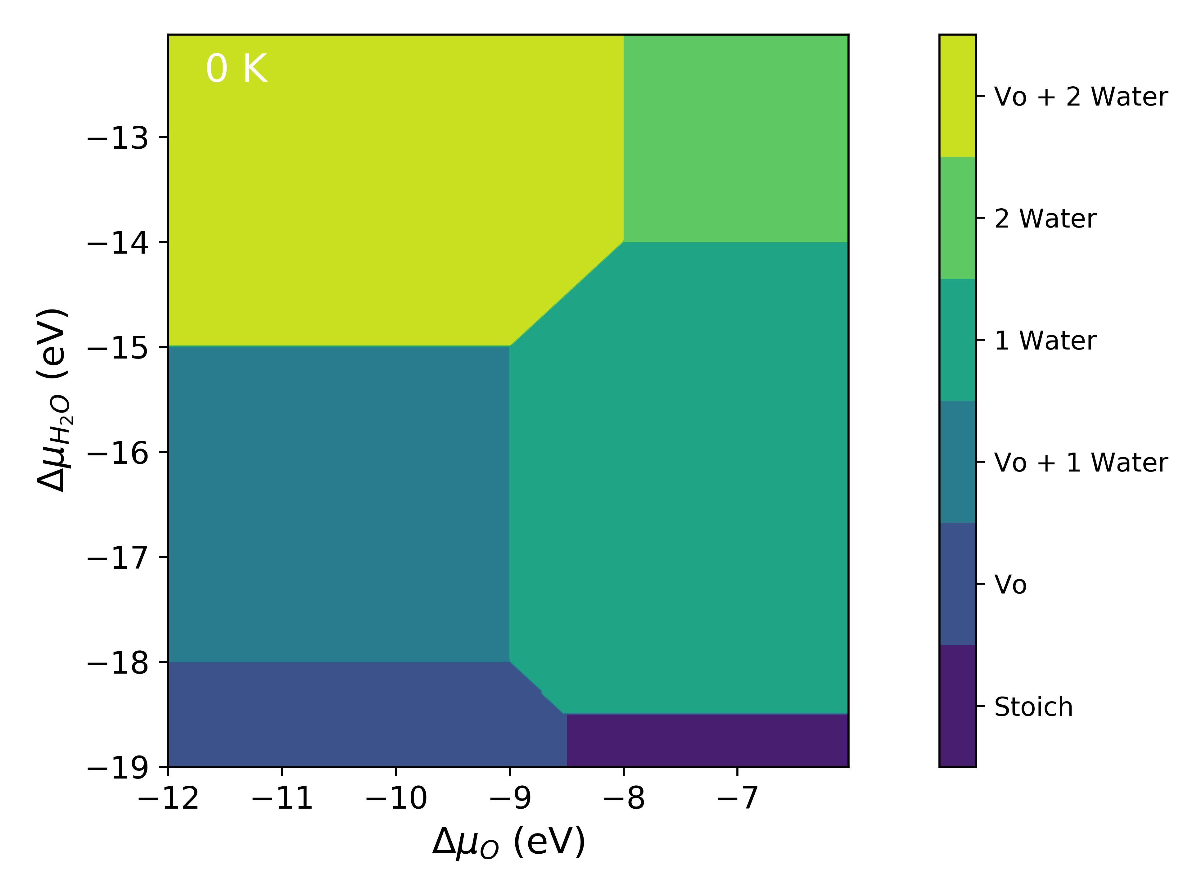
Temperature¶

The previous phase diagram is at 0K. It is possible to use experimental data from the NIST_JANAF database to make the chemical potential a temperature dependent term and thus generate a phase diagram at a temperature (T). Using oxygen as an example, this is done according to

$\gamma_{Surf} = \frac{1}{2A} \Bigg( E_{TiO_2}^{slab} - \frac{nTi_{Slab}}{nTi_{Bulk}} E_{TiO_2}^{Bulk} \Bigg) - \Gamma_O \mu_O - \Gamma_{H_2O} \mu_{H_2O} - n_O \mu_O (T) - n_{H_2O} \mu_{H_2O} (T)$

where

$\mu_O (T) = \frac{1}{2} \mu_O (T) (0 K , DFT) + \frac{1}{2} \mu_O (T) (0 K , EXP) + \frac{1}{2} \Delta G_{O_2} ( \Delta T, Exp),$

$\mu_O$ (T) (0 K , DFT) is the 0K free energy of an isolated oxygen molecule evaluated with DFT, $\mu_O$ (T) (0 K , EXP) is the 0 K experimental Gibbs energy for oxygen gas and $Delta$ $G_{O_2}$ ( $\Delta$ T, Exp) is the Gibbs energy defined at temperature T as

$\Delta G_{O_2} ( \Delta T, Exp) = \frac{1}{2} [H(T, {O_2}) - H(0 K, {O_2})] - \frac{1}{2} T[S(T, {O_2}])$

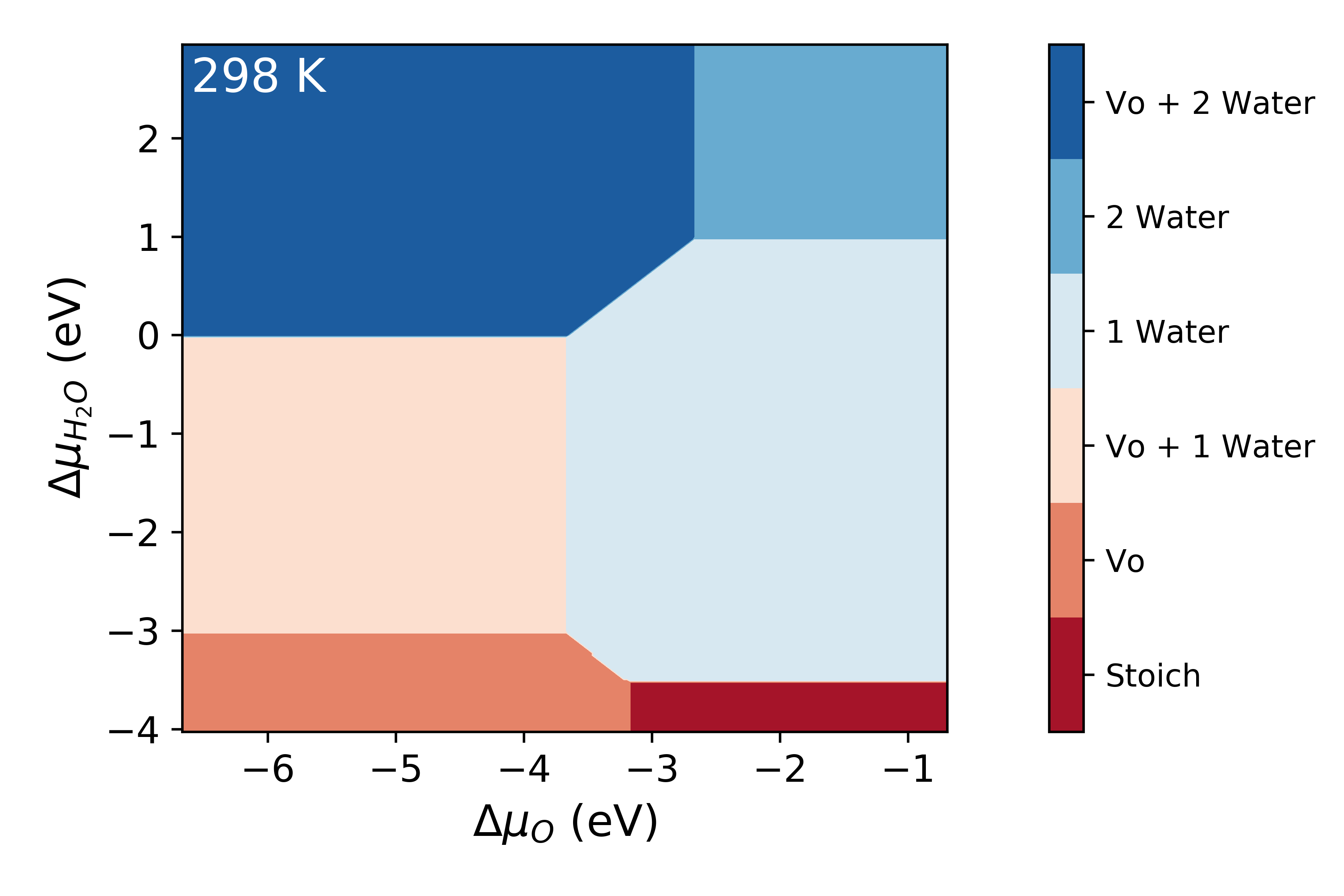
surfinpy has a built in function to read a NIST_JANAF table and calculate this temperature_correction for you. In the following example you will also see an example of how you can tweak the style and colourmap of the plot.

from surfinpy import mu_vs_mu

Oxygen_exp = mu_vs_mu.temperature_correction("O2.txt", 298)
Water_exp = mu_vs_mu.temperature_correction("H2O.txt", 298)

Oxygen_corrected = (-9.08 + -0.86 + Oxygen_exp)
Water_corrected = -14.84 + 0.55 + Water_exp

system =  mu_vs_mu.calculate(data, bulk, deltaX, deltaY,
                             x_energy=Oxygen_corrected,
                             y_energy=Water_corrected)
system.plot_phase(temperature=298, set_style="fast",
                  colourmap="RdBu")

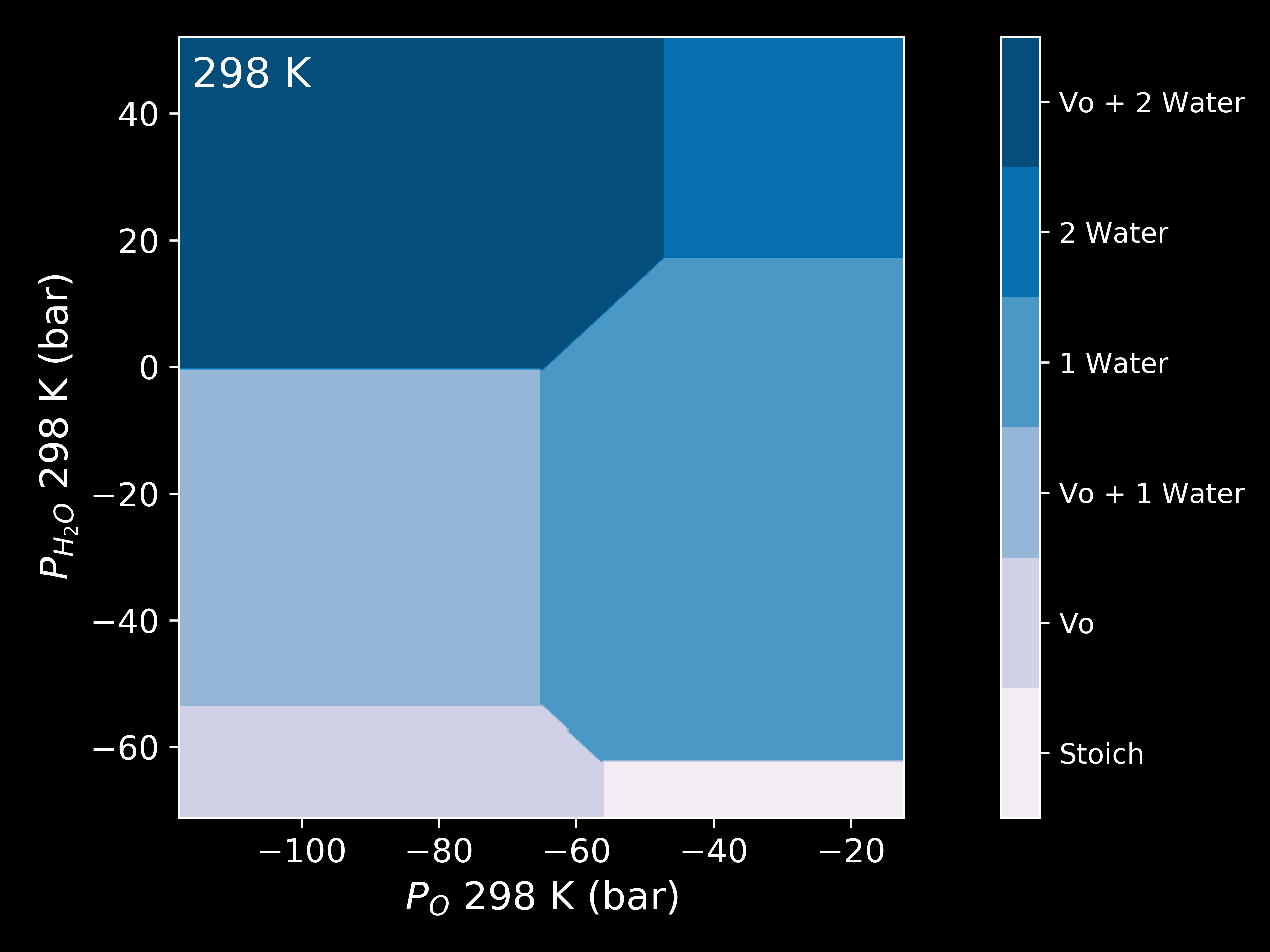
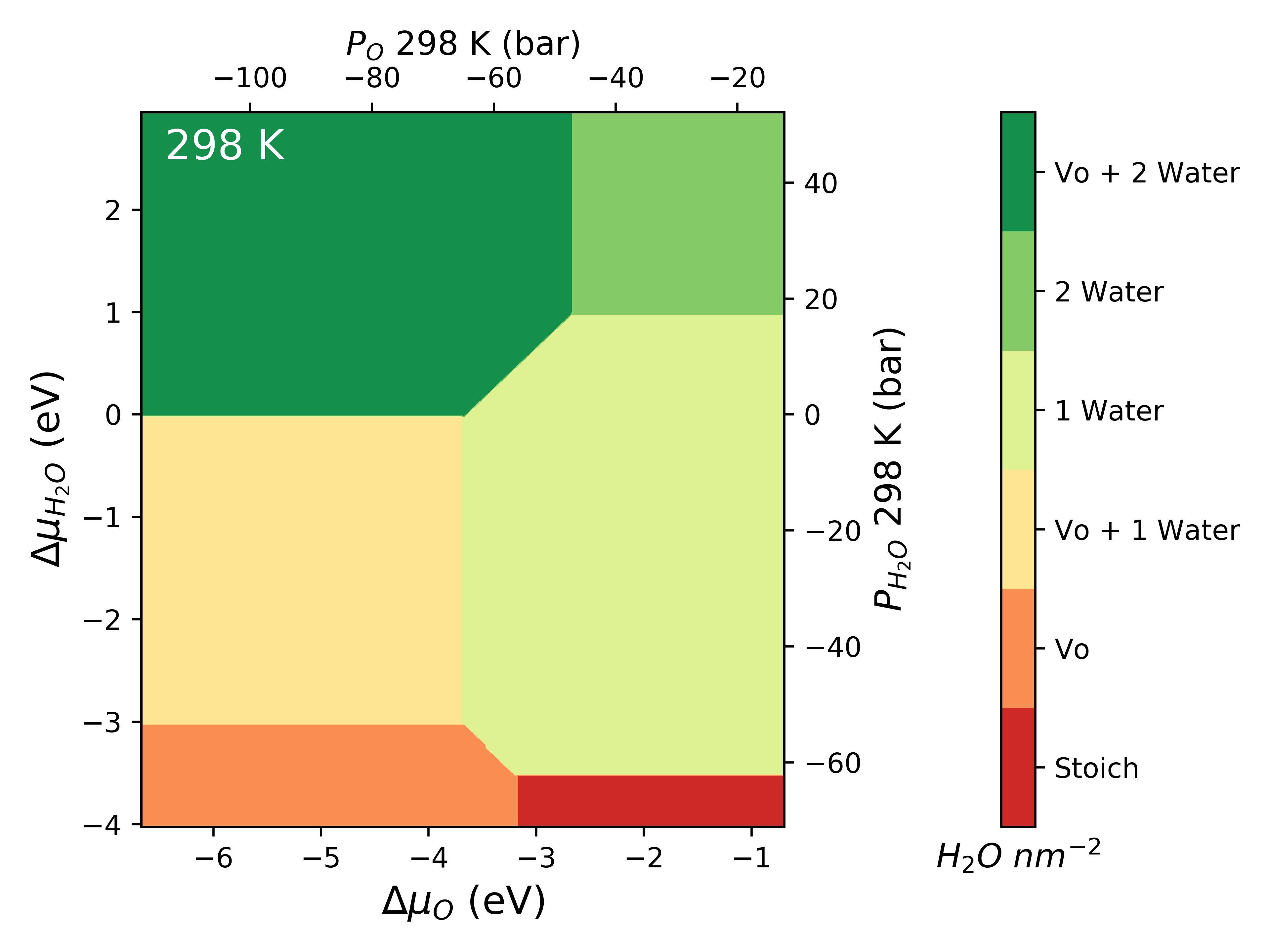
Pressure¶

The chemical potential can be converted to pressure values according to

$P = \frac{\mu_O}{k_B T}$

where P is the pressure, $\mu$ is the chemical potential of oxygen, $k_B$ is the Boltzmnann constant and T is the temperature.

from surfinpy import mu_vs_mu

Oxygen_exp = mu_vs_mu.temperature_correction("O2.txt", 298)
Water_exp = mu_vs_mu.temperature_correction("H2O.txt", 298)

Oxygen_corrected = (-9.08 + -0.86 + Oxygen_exp)
Water_corrected = -14.84 + 0.55 + Water_exp

system =  mu_vs_mu.calculate(data, bulk, deltaX, deltaY,
                             x_energy=Oxygen_corrected,
                             y_energy=Water_corrected)
system.plot_mu_p(output="Example_ggrd", colourmap="RdYlGn",
                 temperature=298)

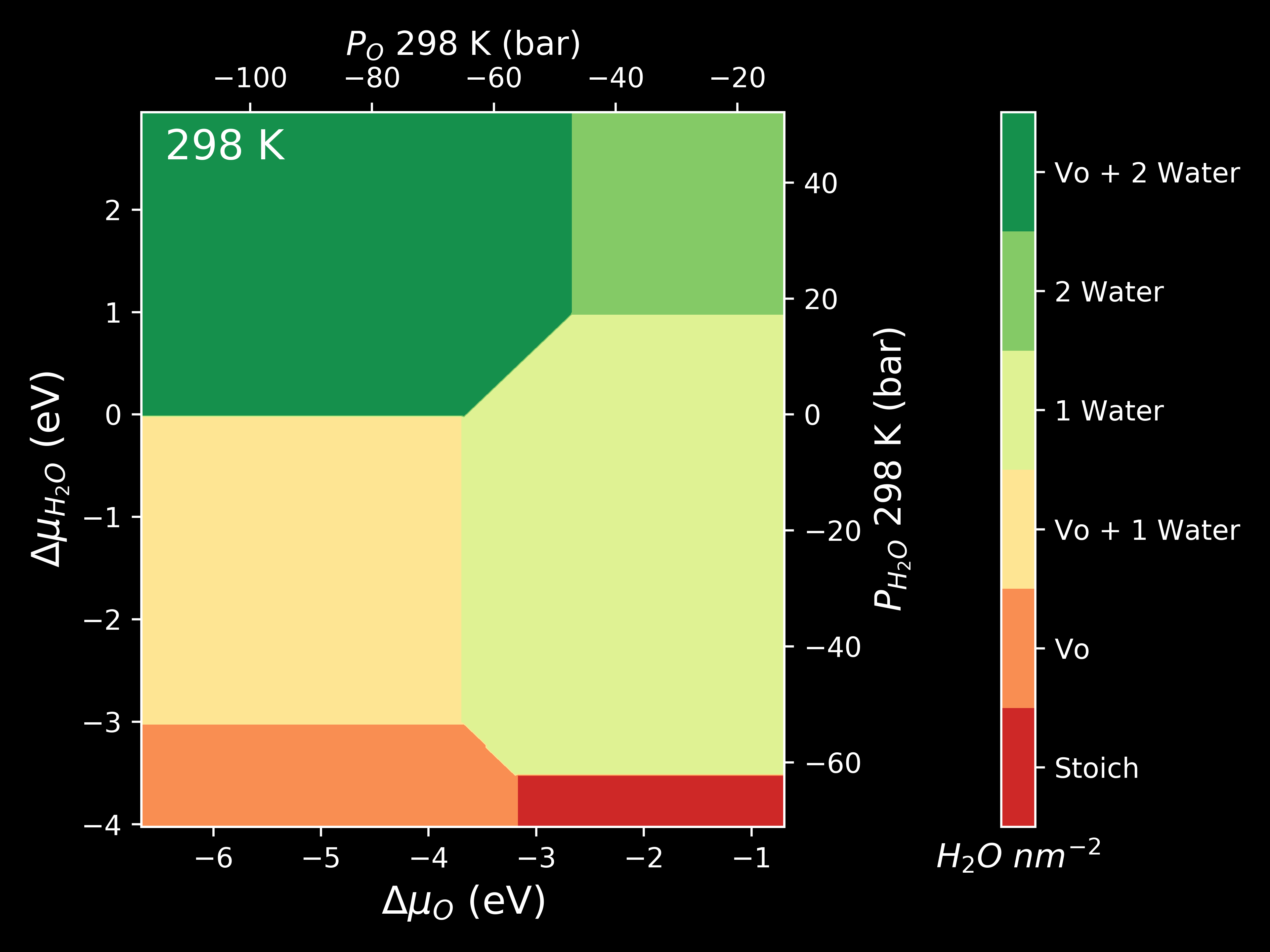
system.plot_mu_p(output="Example_ggrd",
                 set_style="dark_background",
                 colourmap="RdYlGn",
                 temperature=298)

system.plot_pressure(output="Example_dark_rdgn",
                     set_style="dark_background",
                     colourmap="PuBu",
                     temperature=298)