Vibrational Entropy¶

In this example we will expand this methodology to calculate the vibrational properties for solid phases (i.e. zero point energy, vibrational entropy) and include these values in the generation of the phase diagrams. This allows for a more accurate calculation of phase diagrams without the need to include experimental corrections for solid phases.

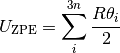
As with previous examples, the standard free energy varies significantly with temperature, and as DFT simulations are designed for condensed phase systems, we use experimental data to determine the temperature dependent free energy term for gaseous species obtained from the NIST database. In addition we also calculate the vibrational properties for the solid phases modifying the free energy (G) for solid phases to be;

$\Delta G_f = U_0 + U_{\text{ZPE}} + A_{\text{vib}}$

$U_0$ is the calculated internal energy from a DFT calculation, $U_{ZPE}$ is the zero point energy and $S_{vib}$ is the vibrational entropy.

$U_{\text{ZPE}} = \sum_i^{3n} \frac{R \theta_i}{2}$

where $A_{vib}$ is the vibrational Helmholtz free energy and defined as;

$A_{\text{vib}} = \sum_i^{3n} RT \ln{(1-e^{-\theta_i/T})}$

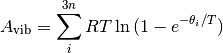
3n is the total number of vibrational modes, n is the number of species and $\theta_i$ is the characteristic vibrational temperature (frequency of the vibrational mode in Kelvin).

$\theta_i = \frac{h\nu_i}{k_B}$

from surfinpy import bulk_mu_vs_mu as bmvm
from surfinpy import utils as ut
from surfinpy import data

temperature_range = [298, 299]

bulk = data.ReferenceDataSet(cation = 1, anion = 1, energy = -92.0, funits = 10, file = 'bulk_vib.yaml', entropy=True, zpe=True, temp_range=temperature_range)

In addition to entropy and zpe keyword you must provide the a file containing the vibrational modes and number of formula units used in taht calculations. You must create the yaml file using the following format

F-Units : number
Frequencies :
- mode1
- mode2

Vibrational modes can be calculated via a density functional pertibation calculation or via the phonopy code.

Bulk = data.DataSet(cation = 10, x = 0, y = 0, energy = -92,
                  label = "Bulk", entropy = True, zpe=True, file = 'ref_files/bulk_vib.yaml',
                  funits = 10, temp_range=temperature_range)

A = data.DataSet(cation = 10, x = 5, y = 20, energy = -468,
                  label = "A", entropy = True, zpe=True, file = 'ref_files/A_vib.yaml',
                  funits = 5, temp_range=temperature_range)

B = data.DataSet(cation = 10, x = 0, y = 10, energy = -228,
                  label = "B", entropy = True, zpe=True, file = 'ref_files/B_vib.yaml',
                  funits =  10, temp_range=temperature_range)

C = data.DataSet(cation = 10, x = 10, y = 30, energy = -706,
                  label = "C", entropy = True, zpe=True, file = 'ref_files/C_vib.yaml',
                  funits = 10, temp_range=temperature_range)

D = data.DataSet(cation = 10, x = 10, y = 0, energy = -310,
                  label = "D", entropy = True, zpe=True,  file = 'ref_files/D_vib.yaml',
                  funits =  10, temp_range=temperature_range)

E = data.DataSet(cation = 10, x = 10, y = 50, energy = -972,
                  label = "E", entropy = True, zpe=True, file = 'ref_files/E_vib.yaml',
                  funits =  10, temp_range=temperature_range)

F = data.DataSet(cation = 10, x = 8, y = 10, energy = -398,
                  label = "F", entropy = True, zpe=True, file = 'ref_files/F_vib.yaml',
                  funits =  2, temp_range=temperature_range)


data = [Bulk, A, B, C, D, E, F]

x_energy=-20.53412969
y_energy=-12.83725889


CO2_exp = ut.fit_nist("CO2.txt")[298]
Water_exp = ut.fit_nist("H2O.txt")[298]

CO2_corrected = x_energy + CO2_exp
Water_corrected = y_energy + Water_exp

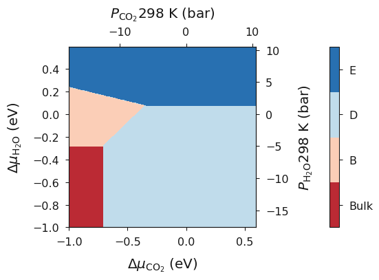
deltaX = {'Range': [ -1, 0.6],  'Label': 'CO_2'}
deltaY = {'Range': [ -1, 0.6], 'Label': 'H_2O'}

temp_298 = bmvm.calculate(data, bulk, deltaX, deltaY, CO2_corrected, Water_corrected)
ax = temp_298.plot_mu_p(temperature=298, set_style="fast", colourmap="RdBu")

Temperature¶

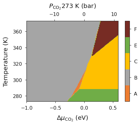
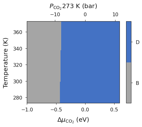
In tutorial 5 we showed how SurfinPy can be used to calculate the vibrational entropy and zero point energy for solid phases and in tutorial 4 we showed how a temperature range can be used to calculate the phase diagram of temperature as a function of presure. In this example we will use both lesson from these tutorials to produce a phase diagram of temperature as a function of pressure including the vibrational properties for solid phases. Again this produces results which are easily compared to experimental values in addition to increasing the level of theory used.

import matplotlib.pyplot as plt
from surfinpy import bulk_mu_vs_mu as bmvm
from surfinpy import utils as ut
from surfinpy import bulk_mu_vs_t as bmvt
from surfinpy import data
import numpy as np

colors = ['#5B9BD5', '#4472C4', '#A5A5A5', '#772C24', '#ED7D31', '#FFC000', '#70AD47']

temperature_range = [273, 373]

bulk = data.ReferenceDataSet(cation = 1, anion = 1, energy = -92.0, funits = 10, file = 'bulk_vib.yaml', entropy=True, zpe=True, temp_range=temperature_range)


Bulk = data.DataSet(cation = 10, x = 0, y = 0, energy = -92., color=colors[0],
                label = "Bulk", entropy = True, zpe=True, file = 'ref_files/bulk_vib.yaml',
                funits = 10, temp_range=temperature_range)

D = data.DataSet(cation = 10, x = 10, y = 0, energy = -310.,  color=colors[1],
                label = "D", entropy = True, zpe=True,  file = 'ref_files/D_vib.yaml',
                funits =  10, temp_range=temperature_range)

B = data.DataSet(cation = 10, x = 0, y = 10, energy = -227.,  color=colors[2],
                label = "B", entropy = True, zpe=True, file = 'ref_files/B_vib.yaml',
                funits =  10, temp_range=temperature_range)

F = data.DataSet(cation = 10, x = 8, y = 10, energy = -398.,  color=colors[3],
                label = "F", entropy = True, zpe=True, file = 'ref_files/F_vib.yaml',
                funits =  2, temp_range=temperature_range)

A = data.DataSet(cation = 10, x = 5, y = 20, energy = -467.,  color=colors[4],
                label = "A", entropy = True, zpe=True, file = 'ref_files/A_vib.yaml',
                funits = 5, temp_range=temperature_range)


C = data.DataSet(cation = 10, x = 10, y = 30, energy = -705.,  color=colors[5],
                label = "C", entropy = True, zpe=True, file = 'ref_files/C_vib.yaml',
                funits = 10, temp_range=temperature_range)

E = data.DataSet(cation = 10, x = 10, y = 50, energy = -971.,  color=colors[6],
                label = "E", entropy = True, zpe=True, file = 'ref_files/E_vib.yaml',
                funits =  10, temp_range=temperature_range)

data = [Bulk, A, B, C,  D, E, F]

deltaX = {'Range': [ -1, 0.6],  'Label': 'CO_2'}
deltaZ = {'Range': [ 273, 373], 'Label': 'Temperature'}
x_energy=-20.53412969
y_energy=-12.83725889
mu_y = 0


exp_x = ut.temperature_correction_range("CO2.txt", deltaZ)
exp_y = ut.temperature_correction_range("H2O.txt", deltaZ)

system = bmvt.calculate(data, bulk, deltaX, deltaZ, x_energy, y_energy, mu_y, exp_x, exp_y)
ax = system.plot_mu_vs_t_vs_p(temperature=273)

When investigating the phase diagram for certain systems it could be beneficial to remove a kinetically inhibited but thermodynamically stable phase to investigate the metastable phase diagram. Within SurfinPy this can be acheived via recreating the data list without the phase in question then recalculating the phse diagram, as below.

data = [Bulk, A, B, C, E, F]

system = bmvt.calculate(data, bulk, deltaX, deltaZ, x_energy, y_energy, mu_y, exp_x, exp_y)
ax = system.plot_mu_vs_t_vs_p(temperature=273)